Cassini Position Example
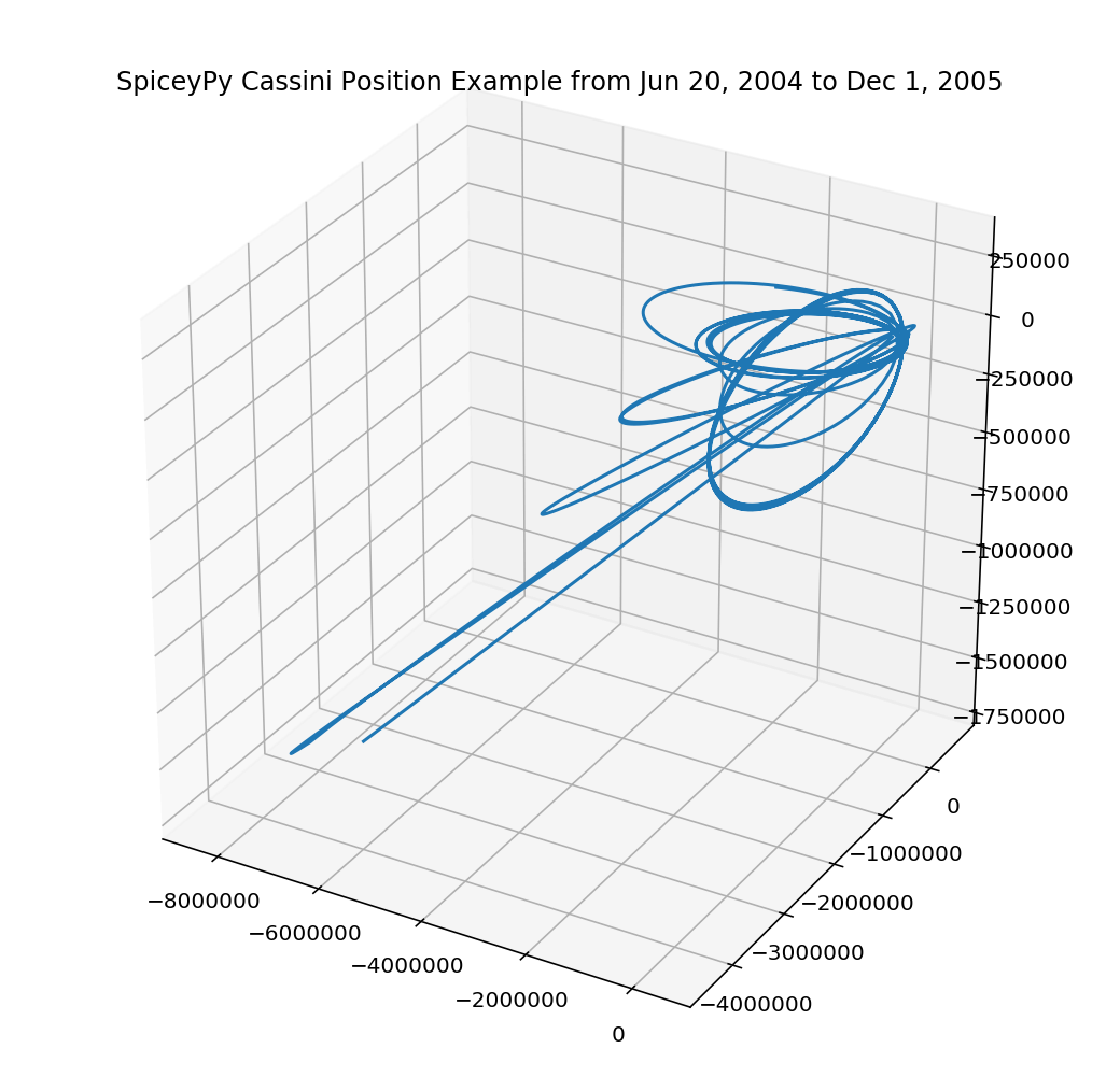
Below is an interactive example that uses spiceypy to plot the position of the Cassini spacecraft relative to the barycenter of Saturn.
First import spiceypy and test it out.
'CSPICE_N0067'
We will need to load some kernels. If you are running this example outside of this browser page, you will need to download the following kernels
from the NAIF servers via the links provided. After the kernels have been downloaded, you can define a meta kernel file or simply provide the paths directly to the spiceypy.furnsh method.
For more on defining meta kernels in spice, please consult the Kernel Required Reading.
ET One: 140961664.18440723, ET Two: 186667264.18308285
[140961664.18440723, 140973090.5844069, 140984516.98440656]
the above command will return something like the following:
Help on function spkpos in module spiceypy.spiceypy:

spkpos(
    targ: str,
    et: Union[float, numpy.ndarray],
    ref: str,
    abcorr: str,
    obs: str
) -> Union[Tuple[numpy.ndarray, float], Tuple[numpy.ndarray, numpy.ndarray]]
    Return the position of a target body relative to an observing
    body, optionally corrected for light time (planetary aberration)
    and stellar aberration.

    https://naif.jpl.nasa.gov/pub/naif/misc/toolkit_docs_N0067/C/cspice/spkpos_c.html

    :param targ: Target body name.
    :param et: Observer epoch in seconds past J2000 TDB.
    :param ref: Reference frame of output position vector.
    :param abcorr: Aberration correction flag.
    :param obs: Observing body name.
    :return:
            Position of target in km,
            One way light time between observer and target in seconds.
Positions:
[-5461446.61080924 -4434793.40785864 -1200385.93315424]
Light Times:
23.8062238783
We will use matplotlib's 3D plotting to visualize Cassini's coordinates. We first convert the positions list to a 2D numpy array for easier indexing in the plot.